Chapter 4 Initialization
So far, we’ve seen how to move from one basic feasible solution to an adjacent one with a higher objective value. To have a complete algorithm for solving standard linear programs, we still need a method that finds some BFS. If we’re lucky, the origin is a basic feasible solution and we can start our simplex method here. However, this is not always the case. The following proposition follows easily from definitions.
Proposition 4.1 The origin is a basic feasible solution of the standard linear program (2.1) if and only if \(b_i \ge 0\) for all \(1 \le i \le m.\)
When the origin is not a BFS, we need a process to find one. This is called the Initialization Phase or Phase I. We will do this by creating an auxiliary linear program.
4.1 Auxiliary Linear Program
Definition 4.1 We say that a linear program is feasible if its feasible region is non-empty.
The initialization phase determines if a standard linear program is feasible and if it is then it finds a BFS by solving the following auxiliary linear program.
Definition 4.2 The auxiliary linear program of the standard linear program (2.1) is defined as follows: \[\begin{equation} \begin{array}{lrrrrrrrrrrr} \mbox{maximize: } & & & & & & & & - & x_0 & \\ \mbox{subject to: } & & & a_{11} x_1 & + & \dots & + & a_{1n} x_n & - &x_0 & \leq & b_1 \\ & & & a_{21} x_1 & + & \dots & + & a_{2n} x_n & - &x_0 & \leq & b_2 \\ & & & & & \vdots & \\ & & & a_{m1} x_1 & + & \dots & + & a_{mn} x_n & - &x_0 & \leq & b_m \\ & & & x_1, & x_2, & \dots &, & x_n & , & x_0 & \geq & 0. \end{array} \tag{4.1} \end{equation}\]
We’re introducing a new variable \(-x_0\), adding \(-x_0\) to each of the constraint LHS, and changing the objective function to \(-x_0\). To understand the auxiliary linear program, we rewrite it in the following non-standard form: \[\begin{equation*} \begin{array}{lrrrrrrrrrrrrr} \mbox{minimize: } & & & & & & & & & & & x_0 & \\ \mbox{subject to: } & & & a_{11} x_1 & + & \dots & + & a_{1n} x_n & \leq & b_1 & + & x_0 \\ & & & a_{21} x_1 & + & \dots & + & a_{2n} x_n & \leq & b_2 & + & x_0 \\ & & & & & \vdots & \\ & & & a_{m1} x_1 & + & \dots & + & a_{mn} x_n & \leq & b_m & + & x_0 \\ & & & x_1, & x_2, & \dots &, & x_n & , & x_0 & \geq & 0 \end{array} \end{equation*}\] We can interpret \(x_0\) as a relaxation of the constraints. Solving the auxiliary linear program is equivalent to asking - “what is the smallest constraint relaxation necessary to make the primary linear program feasible?”. The primary linear program is feasible if and only if no relaxation is necessary. The following exercises make this more precise.
Exercise 4.1 Show that the auxiliary linear program (4.1) is always feasible by explicitly constructing a feasible solution.
Exercise 4.2 Show that the objective values of the auxiliary linear program (4.1) are bounded from above by 0. Using the extreme value theorem, conclude that (4.1) always has an optimal solution.
Finally, the following theorem (proof left as an exercise) establishes an explicit connection between optimal solutions of the auxiliary linear program and feasible solutions of the standard linear program.
Theorem 4.1 Suppose \(x_i = k_i\) for \(0 \le i \le m\) is an optimal solution of the auxiliary linear program (4.1). Then, the standard linear program (2.1) is feasible if and only if \(k_0 = 0\). In this case, \(x_i = k_i\) for \(0 \le i \le m\) is a basic feasible solution of (2.1).
Our problem is now reduced to determining the optimal solution of the auxiliary linear program, which we’ll do using the simplex method itself! However, even for the auxiliary linear program the origin is not necessarily in the feasible region so we cannot use the simplex steps to find an optimal solution. But, in this case, there is a trick to make all the \(b_i \ge 0\) by performing a single elementary row operation as described in the following exercises.
Exercise 4.3 Suppose some \(b_i\) is negative. Without any loss of generality, assume that \(b_1\) is the smallest among all the \(b_i\) (i.e. the most negative). Show that after the pivot step in tableau for the auxiliary linear program (4.1) about the column corresponding to \(x_0\) and the row corresponding to \(w_1\), all the \(b_i\)’s become positive.
To summarize: If the origin is not a vertex of the feasible region, then the method of solving the standard linear program (2.1), starting with Phase I, is as follows:
- Form the auxiliary linear program and its tableau.
- Perform a pivot operation about the entry in the column corresponding to the variable \(x_0\) and the row corresponding to the most negative \(b_i\). This results in a dictionary where all the \(b_i\)’s are now non-negative.
- Solve the auxiliary linear program by repeatedly performing pivot steps.
Suppose \(x_i = k_i\) for \(0 \le i \le m\) is an optimal solution of the auxiliary linear program.
- If \(k_0 \neq 0\), then we halt as the primary linear program is not feasible.
- If \(k_0 = 0\), then we proceed to Phase II. We solve the original linear program starting at the BFS \(x_i = k_i\) for \(1 \le i \le n\) by repeatedly performing pivot steps.
Exercise 4.4 This exercise provides a geometric intuition behind the auxiliary linear program. For each of the following standard linear programs,
\[\begin{equation*} \begin{array}{lrllll} \mbox{maximize:} & x \\ \mbox{subject to:} & -x & \le & -1 \\ & x & \ge & 0 \end{array} \end{equation*}\]
\[\begin{equation*} \begin{array}{lrllll} \mbox{maximize:} & x \\ \mbox{subject to:} & x & \le & -1 \\ & x & \ge & 0 \end{array} \end{equation*}\]
- Form the auxiliary linear program. Use \(y\) as the auxiliary variable.
- Draw the feasible region of the auxiliary linear program and label the constraints using slack variables.
- Solve the auxiliary linear program using geometry.
4.2 Combined tableau
At the end of Phase I, we need to calculate the dictionary at the basic feasible solution \(x_i = k_i\) for \(1 \le i \le n\). We can avoid this recalculation by manipulating a combined tableau which contains information about both the auxiliary and the primary linear programs.
Definition 4.3 The combined tableau is defined as follows: \[\begin{equation*} \begin{array}{rrrrrrrrrrrr|l} a_{11} & & \dots & & a_{1n} & 1 & & & & & & -1 &b_1\\ a_{21} & & \dots & & a_{2n} & & & 1 & & & & -1 &b_2\\ & & & & & \vdots & & & & & & \vdots & \vdots \\ a_{m1} & & \dots & & a_{mn} & & & & & & 1 & -1 &b_m\\ \hline c_1 & & \dots & & c_{n} & 0 & & 0 & \dots & & 0 & 0 & -c_0\\ \hline 0 & & \dots & & 0 & 0 & & 0 & \dots & & 0 & -1 & 0 \end{array} \end{equation*}\]
The second to last row of the tableau corresponds to the objective function of the primary linear program and the last row corresponds to the objective of the auxiliary linear program. The second to last column corresponds to the variable \(x_0\).
We use the combined tableau to first perform Phase I and then delete the auxiliary objective and the variable \(x_0\) and proceed on to Phase II using the rest of the tableau.
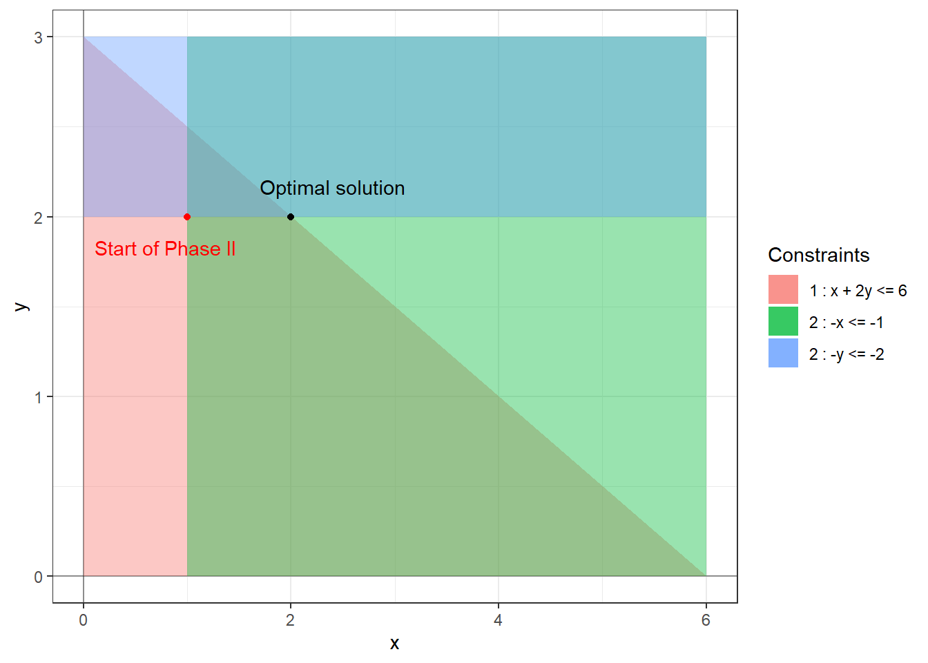
Example 4.1 Consider the following linear program:
\[\begin{equation*}
\begin{array}{rrrrrl}
\mbox{maximize:} & x & + & y \\
\mbox{subject to:}
& x & + & 2y & \le & 6 \\
& -x & & & \le & -1 \\
& & & -y & \le & -2 \\
& x & , & y & \ge & 0.
\end{array}
\end{equation*}\]
As \(b_2\) and \(b_3\) are negative, \((0,0)\) is not feasible and we need to start with Phase I. We form the combined tableau:
\[\begin{equation*}
\begin{array}{rrrrrr|r}
1 & 2 & 1 & 0 & 0 & -1 & 6 \\
-1 & 0 & 0 & 1 & 0 & -1 & -1 \\
0 & -1 & 0 & 0 & 1 & \boxed{-1} & -2 \\ \hline
1 & 1 & 0 & 0 & 0 & 0 & 0 \\ \hline
0 & 0 & 0 & 0 & 0 & -1 & 0
\end{array}
\end{equation*}\]
The first pivot is in the column corresponding to the variable \(x_0\) and the row corresponding to the most negative \(b_i\) (which is \(b_3 = -2\)). This results in the following combined tableau:
\[\begin{equation*}
\begin{array}{rrrrrr|r}
1 & 3 & 1 & 0 & -1 & 0 & 8 \\
-1 & 1 & 0 & 1 & -1 & 0 & 1 \\
0 & 1 & 0 & 0 & -1 & 1 & 2 \\ \hline
1 & 1 & 0 & 0 & 0 & 0 & 0 \\ \hline
0 & 1 & 0 & 0 & -1 & 0 & 2
\end{array}
\end{equation*}\]
We then continue performing pivot steps to find the solution:
\[\begin{equation*}
\begin{array}{rrrrrr|r}
0 & 0 & 1 & 1 & 2 & -4 & 1 \\
0 & 1 & 0 & 0 & -1 & 1 & 2 \\
1 & 0 & 0 & -1 & 0 & 1 & 1 \\ \hline
0 & 0 & 0 & 1 & 1 & -2 & -3 \\ \hline
0 & 0 & 0 & 0 & 0 & -1 & \mathbf{0}
\end{array}
\end{equation*}\]
We see that the optimal value is 0 and hence the primary linear program is feasible. We then remove the auxiliary objective and coefficient to get the following tableau for the primary linear program:
\[\begin{equation*}
\begin{array}{rrrrr|r}
0 & 0 & 1 & \boxed{1} & 2 & 1 \\
0 & 1 & 0 & 0 & -1 & 2 \\
1 & 0 & 0 & -1 & 0 & 1 \\ \hline
0 & 0 & 0 & 1 & 1 & -3
\end{array}
\end{equation*}\]
Continuing with the simplex method we get the following final tableau
\[\begin{equation*}
\begin{array}{rrrrr|r}
0 & 0 & 1 & 1 & 2 & 1 \\
0 & 1 & 0 & 0 & -1 & 2 \\
1 & 0 & 1 & 0 & 2 & 2 \\ \hline
0 & 0 & -1 & 0 & -1 & -4
\end{array}
\end{equation*}\]
The final non-basic variables are \(w_1\) and \(w_3\), the basic variables are \(x\), \(y\), \(w_2\) with values \(2\), \(2\), \(1\), respectively, and the optimal objective value is \(4\). The following figure shows the starting and ending basic feasible solutions for Phase II.