Day 2 - Norms and Estimators
Canada/USA Mathcamp 2026
From Exact to Approximate Fits
In the previous lecture, we saw that fitting a polynomial exactly through all data points leads to overfitting—the estimates become extremely sensitive to small changes in the data. The solution is to allow approximate fits, where our model doesn’t pass through every point exactly.
Instead of requiring y_i = f(x_i), we introduce residuals \epsilon_1, \epsilon_2, \ldots, \epsilon_n and write
y_i = f(x_i) + \epsilon_i, \quad \text{for } i = 1, 2, \ldots, n.
The residual \epsilon_i measures how much the model prediction f(x_i) differs from the observed value y_i. A good model should make the residuals “small”—but what exactly does “small” mean for a collection of n numbers?
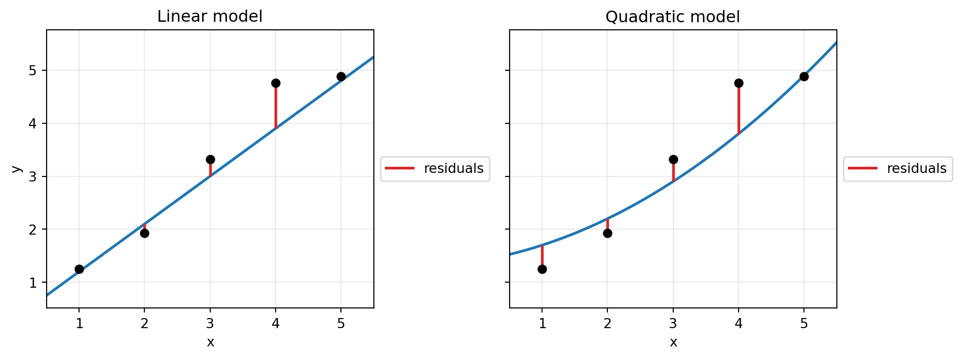
The plots below show two different models fit to the same data. The vertical segments highlight the residuals: the gap between each observed data point and the model’s prediction.
This question leads us to a fundamental principle:
TipThe Core Idea: Estimation = Minimization
Estimating a quantity from data is equivalent to minimizing the residuals with respect to a chosen notion of “size.”
Different notions of size lead to different estimators. This is the foundation of modern data science, machine learning, and AI. For example, training a neural network means choosing a loss function (a way to measure residual size) and minimizing it with respect to the network’s parameters.
Today we’ll explore this principle through the simplest possible estimation problem: estimating a constant from repeated measurements.
Estimating a Constant
Suppose you measure the gravitational acceleration g at Earth’s surface. Due to measurement error, each trial gives a slightly different value. Here are 10 measurements (in m/s²):
Measurements: [ 9.986  9.85   9.908 10.034  9.997  9.712  9.905  9.795  9.8    9.851]
Min: 9.712, Max: 10.034
What single value best represents the “true” gravitational acceleration?
We want to find a constant g such that
g_i = g + \epsilon_i, \quad \text{for } i = 1, 2, \ldots, n,
where the residuals \epsilon_i = g_i - g are as “small” as possible. We use \widehat{g} to denote the estimate calculated from the data (the minimizer) and g to denote a candidate value we’re optimizing over.
NoteConnection to Regression
This is a regression problem in disguise! We’re fitting a “degree 0 polynomial” (a constant function) to the data. The techniques we develop here generalize to fitting lines, parabolas, and more complex models.
Measuring Size: Norms
To make “small residuals” precise, we need to measure the size of the residual vector
\vec{\epsilon} = \begin{bmatrix}\epsilon_1 \\ \epsilon_2 \\ \vdots \\ \epsilon_n\end{bmatrix} \in \mathbb{R}^n.
A function that measures vector size is called a norm.
Definition and Properties
A norm on \mathbb{R}^n is a function \|\cdot\|: \mathbb{R}^n \to \mathbb{R} satisfying:
- Positivity: \|\vec{x}\| \geq 0 for all \vec{x}, with \|\vec{x}\| = 0 if and only if \vec{x} = \vec{0}.
- Scaling: \|\alpha \vec{x}\| = |\alpha| \cdot \|\vec{x}\| for all scalars \alpha and vectors \vec{x}.
- Triangle inequality: \|\vec{x} + \vec{y}\| \leq \|\vec{x}\| + \|\vec{y}\| for all \vec{x}, \vec{y}.
TipWhy these axioms?
- Positivity ensures size is non-negative and only the zero vector has zero size.
- Scaling says stretching a vector by factor \alpha stretches its size by |\alpha|.
- Triangle inequality says the direct path is never longer than going through an intermediate point. This property enables calculus with norms.
The L^p Family
The most important norms are the L^p norms, defined for p \geq 1:
\|\vec{x}\|_p = \left( |x_1|^p + |x_2|^p + \cdots + |x_n|^p \right)^{1/p}
Different values of p weight errors differently:
- Small p: treats all errors more equally
- Large p: increasingly dominated by the largest errors
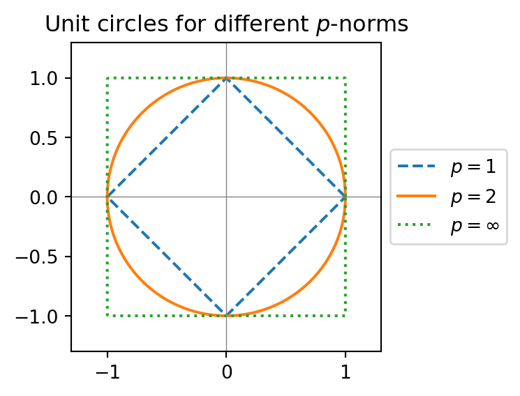
The plot below shows the unit circles \{\vec{x} \in \mathbb{R}^2 : \|\vec{x}\|_p = 1\} for different values of p.
Three Estimators
We now apply three different norms to our estimation problem and discover that each leads to a familiar statistic.
L^2 Norm
The L^2 norm is the Euclidean distance:
\|\vec{\epsilon}\|_2 = \sqrt{\epsilon_1^2 + \epsilon_2^2 + \cdots + \epsilon_n^2}
Because squaring amplifies large values, the L^2 norm penalizes large errors heavily.
ImportantL^2 Estimation Problem
Find the value \widehat{g}_2 that minimizes
\sqrt{(g - g_1)^2 + (g - g_2)^2 + \cdots + (g - g_n)^2}
over all possible values of g. This minimizer is called the ordinary least squares (OLS) estimate.
NoteExercises: L^2 Estimation
Exercise 1: For data g_1 = -2, g_2 = -1, g_3 = 0, g_4 = 1, g_5 = 4, find the OLS estimate \widehat{g}_2.
Exercise 2:
- Show that if h(x) \geq 0 for all x, then minimizing h(x) is equivalent to minimizing h(x)^2.
- For general data g_1, g_2, \ldots, g_n, find the OLS estimate \widehat{g}_2.
L^1 Norm
The L^1 norm is the Manhattan distance:
\|\vec{\epsilon}\|_1 = |\epsilon_1| + |\epsilon_2| + \cdots + |\epsilon_n|
Unlike L^2, the L^1 norm treats all errors proportionally—an error twice as large contributes exactly twice as much.
ImportantL^1 Estimation Problem
Find the value \widehat{g}_1 that minimizes
|g - g_1| + |g - g_2| + \cdots + |g - g_n|
over all possible values of g. This minimizer is called the least absolute deviations (LAD) estimate.
NoteExercises: L^1 Estimation
Exercise 3: For data g_1 = -2, g_2 = -1, g_3 = 0, g_4 = 1, g_5 = 4, find the LAD estimate \widehat{g}_1.
Exercise 4: For sorted data g_1 \leq g_2 \leq \cdots \leq g_n with n odd, find \widehat{g}_1.
Exercise 5: For sorted data with n even, find \widehat{g}_1. (The answer may not be unique!)
L^\infty Norm
As p \to \infty, the L^p norm converges to the maximum norm:
\|\vec{\epsilon}\|_\infty = \max(|\epsilon_1|, |\epsilon_2|, \ldots, |\epsilon_n|)
This norm only cares about the single worst error—all other errors are irrelevant.
ImportantL^\infty Estimation Problem
Find the value \widehat{g}_\infty that minimizes
\max(|g - g_1|, |g - g_2|, \ldots, |g - g_n|)
over all possible values of g. This minimizer is called the minimax estimate.
NoteExercises: L^\infty Estimation
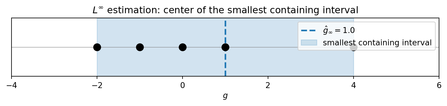
Exercise 6: For data g_1 = -2, g_2 = -1, g_3 = 0, g_4 = 1, g_5 = 4, find \widehat{g}_\infty.
Exercise 7: For sorted data g_1 \leq g_2 \leq \cdots \leq g_n, find a formula for \widehat{g}_\infty.
Geometric interpretation: The L^\infty estimation problem asks: find the smallest interval [g - r, g + r] that contains all the data points. The center of this interval is \widehat{g}_\infty, and its half-width r is the minimized L^\infty norm.
Summary: Three Norms, Three Statistics
We’ve discovered a beautiful unification: three familiar statistics arise from minimizing three different norms.
| Norm | Estimator \widehat{g} | Common Name |
|---|---|---|
| L^2 | \frac{1}{n}\sum_{i=1}^n g_i | Mean |
| L^1 | median of data | Median |
| L^\infty | \frac{\min(g_i) + \max(g_i)}{2} | Midrange |
Let’s verify with our gravitational acceleration data:
         Norm Estimate
    L² (mean)   9.8838
  L¹ (median)   9.8780
L∞ (midrange)   9.8732
   True value   9.8100
All three estimates are close to the true value, but they differ—and they behave very differently when things go wrong. The mean uses all data but is sensitive to outliers; the median is robust to outliers but ignores magnitudes; the midrange only uses extreme values, making it extremely sensitive to outliers.
Which should we prefer? It depends on what we know about our measurement errors. If we trust all measurements equally, the mean is natural. If we suspect some measurements may be wildly incorrect, the median provides protection. In practice, the mean (L^2) dominates—and the next lecture will explain why: it turns out to be the optimal estimator when measurement errors follow a normal distribution.
NoteExercise: Robustness to Outliers
Exercise 8: Consider the data g_1 = -2, g_2 = -1, g_3 = 0, g_4 = 1, g_5 = 4 from the earlier exercises. Suppose the last value was recorded incorrectly as g_5 = 40 instead of g_5 = 4. Recompute all three estimates \widehat{g}_1, \widehat{g}_2, and \widehat{g}_\infty with this corrupted data. Which estimator changed the most? Which changed the least? Explain why.
Looking Ahead
We’ve seen that different norms lead to different estimators. But which norm should we use?
The L^2 norm has a special status. In the next lecture, we’ll introduce the normal distribution and see that:
- If measurement errors follow a normal distribution, then the L^2 estimator is optimal (maximum likelihood).
- This explains why the mean and least squares are ubiquitous in statistics.
We’ll also extend this framework from estimating constants to fitting lines and more complex models.
Additional Exercises
NoteExercises: L^p Norms
The main challenge is verifying the triangle inequality; the other axioms are straightforward. For all the following exercises, you may assume that n = 2 so that \vec{x} = (x_1, x_2) and \vec{y} = (y_1, y_2). The proofs extend to general n by induction.
Exercise 9: Prove that \|\cdot\|_1 satisfies all three norm axioms.
Exercise 10: Prove that \|\cdot\|_2 satisfies all three norm axioms.
Exercise 11: Prove that \|\cdot\|_\infty satisfies all three norm axioms.
Exercise 12:
- Prove that if \|x\| is a norm, then \|x\| ^\circ = k\|x\| is also a norm for any k > 0.
- Prove that if \|x\|' and \|x\|'' are norms, then \|x\|''' = \|x\|' + \|x\|'' is also a norm.
Because of these closure properties, the set of all norms forms a convex cone—it’s closed under positive scaling and addition, but not subtraction.
Exercise 13: Prove that \lim_{p \to \infty} \|\vec{x}\|_p = \max(|x_1|, \ldots, |x_n|). (Hint: Divide by \max(|x_1|, \ldots, |x_n|).)