3 Estimating \(\pi\)
Adjust the slider below to see how the Monte Carlo estimates are calculated for \(\pi\).
Loading interactive visualization...
We begin with a classic Monte Carlo application: estimating the value of \(\pi\) using geometric probability. This example illustrates the core principles of Monte Carlo simulation while providing an intuitive geometric interpretation.
Consider a unit circle inscribed in a square with side length 2, both centered at the origin. The circle has radius \(r = 1\) and area \(A_{\text{circle}} = \pi\), while the square has area \(A_{\text{square}} = 4\). The ratio of these areas is \(\pi/4\).
NoteGeometric Relationships
- Circle: radius \(r = 1\), area \(A_{\text{circle}} = \pi r^2 = \pi\)
- Square: side length \(2r = 2\), area \(A_{\text{square}} = (2r)^2 = 4\)
- Area ratio: \(\frac{A_{\text{circle}}}{A_{\text{square}}} = \frac{\pi}{4}\)
If we randomly sample points uniformly within the square, the probability that any point falls inside the inscribed circle equals this area ratio. This geometric probability provides our pathway to estimating \(\pi\).
To formulate this as a Monte Carlo problem, let \((X, Y)\) be uniformly distributed on \([-1, 1] \times [-1, 1]\) and define the indicator random variable: \[I(X, Y) = \mathbf{1}_{\{X^2 + Y^2 \leq 1\}} = \begin{cases} 1 & \text{if } X^2 + Y^2 \leq 1 \text{ (inside circle)} \\ 0 & \text{if } X^2 + Y^2 > 1 \text{ (outside circle)} \end{cases}\]
The expected value of this indicator function gives us the desired probability: \[\mathbb{E}[I(X, Y)] = P(X^2 + Y^2 \leq 1) = \frac{\text{Area of unit circle}}{\text{Area of square}} = \frac{\pi}{4}\]
Therefore \(\pi = 4\mathbb{E}[I(X, Y)]\), and given \(N\) independent samples \((X_1, Y_1), \ldots, (X_N, Y_N)\), our Monte Carlo estimator is: \[\hat{\pi}_N = 4 \cdot \frac{1}{N}\sum_{i=1}^{N} I(X_i, Y_i) = \frac{4 \cdot \text{(number of points inside circle)}}{N}\]
3.1 Statistical Properties
This estimator possesses several important statistical properties. First, it is unbiased: \[\mathbb{E}[\hat{\pi}_N] = 4\mathbb{E}\left[\frac{1}{N}\sum_{i=1}^{N} I_i\right] = 4\mathbb{E}[I] = 4 \cdot \frac{\pi}{4} = \pi\]
Since \(I \sim \text{Bernoulli}(\pi/4)\), we can compute the variance. The indicator has variance \(\text{Var}(I) = \frac{\pi}{4}(1 - \frac{\pi}{4}) = \frac{\pi(4-\pi)}{16}\), which gives our estimator variance: \[\text{Var}(\hat{\pi}_N) = 16 \cdot \frac{\text{Var}(I)}{N} = \frac{\pi(4-\pi)}{N}\]
The standard error is therefore \(\text{SE}(\hat{\pi}_N) = \sqrt{\frac{\pi(4-\pi)}{N}}\).
ImportantConvergence Rate
The standard error decreases as \(O(1/\sqrt{N})\), which is the typical Monte Carlo convergence rate. To gain one decimal place of accuracy, we need approximately 100 times more samples.
By the Central Limit Theorem, for large \(N\) we have the asymptotic distribution: \[\sqrt{N}(\hat{\pi}_N - \pi) \xrightarrow{d} \mathcal{N}(0, \pi(4-\pi))\]
This provides approximate confidence intervals: \[\hat{\pi}_N \pm z_{\alpha/2} \sqrt{\frac{\pi(4-\pi)}{N}}\]
3.2 Convergence Analysis
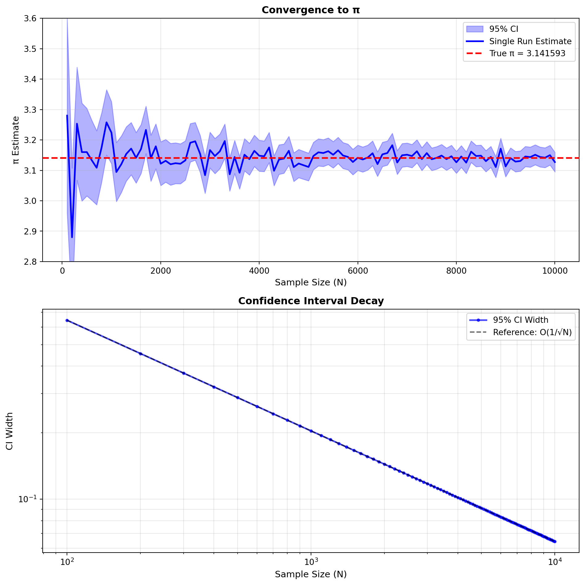
To empirically demonstrate the convergence properties, we generate multiple π estimates for various sample sizes and examine how the confidence intervals narrow as \(N\) increases.
The figure demonstrates that as the sample size \(N\) increases, the mean estimate approaches the true value of \(\pi\) and the confidence interval narrows, confirming the \(O(1/\sqrt{N})\) convergence rate.
TipMonte Carlo Principle
This example demonstrates the fundamental Monte Carlo approach: reformulate a deterministic problem (computing \(\pi\)) as the expectation of a random variable, then estimate that expectation using sample averages.