      Function  True Value  Mean Est   Error  Std Dev  Std Ratio
0       Smooth         2.0    2.0008  0.0008   0.0086          -
1 Oscillatory 2.0 1.9919 0.0081 0.6073 71.006457Monte Carlo integration transforms the problem of computing definite integrals into a sampling problem, making it particularly powerful for high-dimensional integration where traditional methods fail.
Consider the problem of estimating the integral \(\ell = \int_a^b f(x) \, dx\). The key insight is to rewrite this integral as an expectation. If \(X \sim \text{Uniform}(a, b)\), then: \[\int_a^b f(x) \, dx = (b-a) \mathbb{E}[f(X)]\]
This reformulation allows us to estimate the integral using sample averages. Given \(N\) independent samples \(X_1, \ldots, X_N \sim \text{Uniform}(a, b)\), our Monte Carlo estimator is: \[\hat{\ell}_N = \frac{b - a}{N} \sum_{i=1}^{N} f(X_i)\]
We’re approximating the area under \(f(x)\) by averaging function values at random points and scaling by interval width.
The Monte Carlo integration estimator possesses several important statistical properties. First, it is unbiased: \[\begin{aligned} \mathbb{E}[\hat{\ell}_N] &= \frac{b - a}{N} \sum_{i=1}^{N} \mathbb{E}[f(X_i)] = \frac{b - a}{N} \sum_{i=1}^{N} \int_a^b f(x) \frac{1}{b - a} \, dx = \ell \end{aligned}\]
The variance of our estimator is: \[\text{Var}(\hat{\ell}_N) = \frac{(b - a)^2}{N} \cdot \sigma^2_f\] where \(\sigma^2_f = \text{Var}(f(X))\) is the variance of \(f(X)\) under the uniform distribution.
Standard Error: \(\text{SE} = \frac{(b-a)\sigma_f}{\sqrt{N}}\)
Convergence Rate: \(O(1/\sqrt{N})\) regardless of dimension
CLT: \(\sqrt{N}(\hat{\ell}_N - \ell) \xrightarrow{d} \mathcal{N}(0, (b-a)^2\sigma^2_f)\)
Monte Carlo integration’s performance depends heavily on the function’s characteristics. While the convergence rate is theoretically independent of function complexity, practical performance varies significantly with function smoothness and oscillatory behavior.
Functions with high-frequency oscillations present particular challenges for Monte Carlo methods because random sampling may miss important features or fail to adequately capture rapid variations. This example compares Monte Carlo integration performance on two trigonometric functions with dramatically different oscillation frequencies, illustrating how function characteristics affect integration accuracy and convergence behavior.
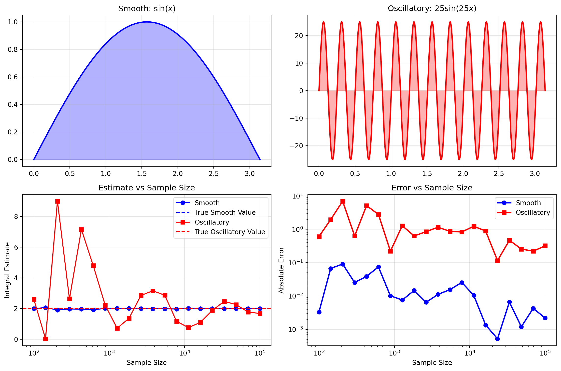
The following example integrates two functions over the interval \([0, \pi]\):
Smooth decay: \(f_1(x) = \sin(x)\) — a smooth, slowly varying function
Oscillatory: \(f_2(x) = 25\sin(25x)\) — a rapidly oscillating function with many periods
Function True Value Mean Est Error Std Dev Std Ratio
0 Smooth 2.0 2.0008 0.0008 0.0086 -
1 Oscillatory 2.0 1.9919 0.0081 0.6073 71.006457The contrast between the smooth \(\sin(x)\) and rapidly oscillating \(25\sin(25x)\) demonstrates why integration difficulty varies. The high-frequency function has many more sign changes and local extrema that random sampling must capture.
The log-log error plot reveals that while both functions follow the expected \(O(1/\sqrt{n})\) convergence rate, the high-frequency function consistently maintains higher absolute errors across all sample sizes. The variance ratio indicates that the oscillatory function’s variance is around 70 times higher than the smooth function’s variance, illustrating how oscillations increase uncertainty in Monte Carlo estimates.
Smooth functions are well-suited for Monte Carlo integration, converging quickly with relatively few samples.
Highly oscillatory functions present challenges, requiring larger sample sizes and exhibiting higher variance.
For oscillatory integrals, consider alternative approaches such as:
This example demonstrates why understanding your function’s characteristics is crucial for effective Monte Carlo integration.
For smooth functions, we can bound the variance using derivative information.
If \(g\) is differentiable on \([a,b]\) with derivative \(g'\), then: \[\text{Var}(g(X)) \leq (b-a)^2 \cdot \max_{x \in [a,b]} |g'(x)|^2\]
Proof. Let \(M = \max_{x \in [a,b]} |g'(x)|\) and \(\mu = \mathbb{E}[g(X)]\).
Since \(g\) is continuous on the compact interval \([a,b]\), it attains its minimum and maximum values. Let \(g_{\min} = \min_{x \in [a,b]} g(x)\) and \(g_{\max} = \max_{x \in [a,b]} g(x)\).
By the mean value theorem, for any two points in \([a,b]\): \[g_{\max} - g_{\min} \leq M(b - a)\]
Since \(\mu = \mathbb{E}[g(X)]\) lies between \(g_{\min}\) and \(g_{\max}\), we have for any \(x \in [a,b]\): \[|g(x) - \mu| \leq g_{\max} - g_{\min} \leq M(b - a)\]
Squaring both sides and taking expectations: \[\text{Var}(g(X)) = \mathbb{E}[(g(X) - \mu)^2] \leq [M(b - a)]^2\]
This gives us the desired bound.
Note that this is a very weak bound and not useful in practice. There are no universal techniques that give us good bounds on \(\text{Var}(g(X))\). In practice, we rely on the heuristic that oscillatory functions are high variance.
One of Monte Carlo integration’s greatest advantages becomes apparent in higher dimensions. While traditional numerical integration methods (like the trapezoidal rule or Simpson’s rule) suffer from the “curse of dimensionality”—requiring exponentially more grid points as dimensions increase—Monte Carlo methods maintain their \(O(1/\sqrt{n})\) convergence rate regardless of dimension.
In \(d\) dimensions, a grid-based method with \(m\) points per dimension requires \(m^d\) total evaluations. For even modest accuracy in high dimensions, this becomes computationally prohibitive. Monte Carlo integration, however, uses the same number of random samples regardless of dimension, making it the method of choice for high-dimensional problems in physics, finance, and machine learning.
The following example demonstrates Monte Carlo integration of the function \(f(\mathbf{x}) = e^{-\|\mathbf{x}\|^2}\) over the unit hypercube \([0,1]^d\) for dimensions \(d = 1, 2, 3, 4, 5\).
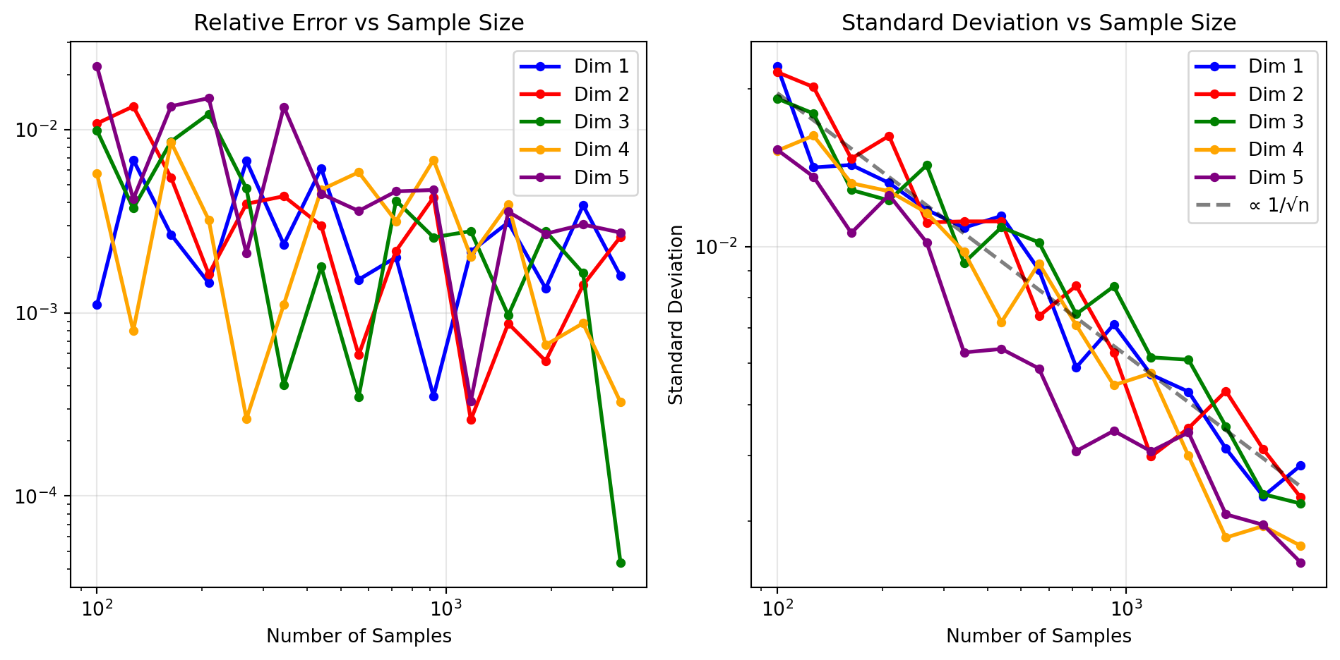
The example reveals several important properties of multidimensional integration:
Dimension-Independent Convergence: The relative error plots demonstrate Monte Carlo’s key advantage - convergence behavior remains consistent across all dimensions, avoiding the curse of dimensionality that plagues grid-based methods.
Theoretical Validation: The standard deviation follows the expected \(1/\sqrt{n}\) scaling (shown by the dashed reference line) regardless of dimension, confirming Monte Carlo’s theoretical foundation.
Constant Computational Cost: Unlike deterministic methods requiring \(n^d\) evaluations, Monte Carlo uses the same number of function evaluations per sample regardless of dimension.
This dimensional robustness makes Monte Carlo indispensable for high-dimensional applications in physics, statistics, and finance where traditional methods become computationally intractable.
Advantages:
High dimensions: Performance doesn’t degrade with dimension
Complex domains: Easy to handle irregular integration regions
Rough functions: Works with discontinuous or highly oscillatory functions
Disadvantages:
Slow convergence: \(O(1/\sqrt{N})\) rate
Random error: Introduces stochastic uncertainty
Low dimensions: Often outperformed by deterministic methods
Practical Considerations:
Sample size: Need large \(N\) for high precision
Function smoothness: Smoother functions → lower variance → better estimates
Variance reduction: Techniques like antithetic variables can improve efficiency
Error estimation: Use sample variance to estimate uncertainty
Monte Carlo integration transforms integration into a sampling problem, making it invaluable for high-dimensional problems where traditional quadrature fails. While it converges slowly, its dimension-independent performance and ability to handle complex functions make it essential for modern computational statistics and machine learning applications.