8 Other Distributions
8.1 Beta Distribution
The Beta distribution is a continuous distribution defined on the interval \([0, 1]\). Let \(X\) be a random variable with Beta distribution with parameters \(\alpha > 0\) and \(\beta > 0\). The probability density function of \(X\) is given by
\[\begin{align*} f(x) = cx^{\alpha-1} (1-x)^{\beta-1}, \quad 0 \leq x \leq 1, \end{align*}\]
where \(c= \frac{(\alpha + \beta - 1)!}{(\alpha-1)!(\beta-1)!}\) is the normalizing constant. (Note that when \(\alpha\) and \(\beta\) are not integers, we use the \(\Gamma\) function as a generalization of the factorial function.)
This is a simple function supported over the interval \([0, 1]\). The Beta distribution is used as a prior distribution in Bayesian statistics. When \(\alpha\) and \(\beta\) are non-integers, the CDF of the Beta distribution does not have a closed-form expression, making inverse transform sampling impractical. Instead, we can use the Beta-Order Statistics connection to sample from the Beta distribution.
Definition 8.1 (Order Statistics): Let \(X_1, X_2, \ldots, X_n\) be independent and identically distributed random variables. The \(k\)-th order statistic, denoted \(X_{(k)}\), is the \(k\)-th smallest value among \(X_1, X_2, \ldots, X_n\).
Theorem 8.1 (Beta-Order Statistics): Let \(U_1, U_2, \ldots, U_n\) be independent random variables with uniform distribution \(U(0, 1)\). Then the random variable \(X = U_{(k)}\) has Beta distribution with parameters \(\alpha = k\) and \(\beta = n - k + 1\).
Proof. We’ll work out a partial proof of the theorem. Let \(X = U_{(k)}\). The cumulative distribution function of \(X\) is given by
\[\begin{align*} F(x) &= \mathbb{P}(U_{(k)} \leq x) \\ &= \mathbb{P}(\text{at least } k \text{ variables among } U_1, U_2, \ldots, U_n \text{ are less than } x) \\ &= \sum_{i=k}^{n} \binom{n}{i} x^i (1-x)^{n-i}. \end{align*}\]
We differentiate both sides to get the probability density function of \(X\):
\[\begin{align*} f(x) &= \frac{d}{dx} F(x) \\ &= \sum_{i=k}^{n} \binom{n}{i} \frac{d}{dx}x^i (1-x)^{n-i} \\ &= \sum_{i=k}^{n} \binom{n}{i} i x^{i-1} (1-x)^{n-i} - \binom{n}{i} (n-i) x^i (1-x)^{n-i-1}. \end{align*}\]
The rest of the proof involves checking that the higher terms in the alternating sum cancel out and only the first term with \(i = k\) remains. \(\blacksquare\)
This theorem gives us a simple algorithm to sample from the Beta distribution:
NoteAlgorithm
- Generate \(n\) random numbers \(u_1, u_2, \ldots, u_n\) from the uniform distribution \(U(0, 1)\).
- Sort the numbers in increasing order \(u_{(1)} \leq u_{(2)} \leq \ldots \leq u_{(n)}\).
- Return \(u_{(k)}\).
8.2 Mixture Distributions
A mixture distribution is a probability distribution that is formed by taking a weighted sum of two or more probability distributions. Let \(X\) be a random variable that is a mixture of distributions \(f_1(x), f_2(x), \ldots, f_n(x)\) with weights \(w_1, w_2, \ldots, w_n\). The probability density function of \(X\) is given by
\[\begin{align*} f(x) = w_1 f_1(x) + w_2 f_2(x) + \ldots + w_n f_n(x). \end{align*}\]
Mixture distributions are used to model complex distributions that cannot be modeled by a single distribution. We can sample from a mixture distribution by first selecting which component distribution to sample from (with probabilities given by the weights), then sampling from that selected distribution.
To sample from a mixture distribution, we can use the following algorithm:
NoteAlgorithm
- Sample from the discrete distribution with probabilities \([w_1, w_2, \ldots, w_n]\) to select a component distribution.
- Sample from the selected component distribution.
- Return the sample.
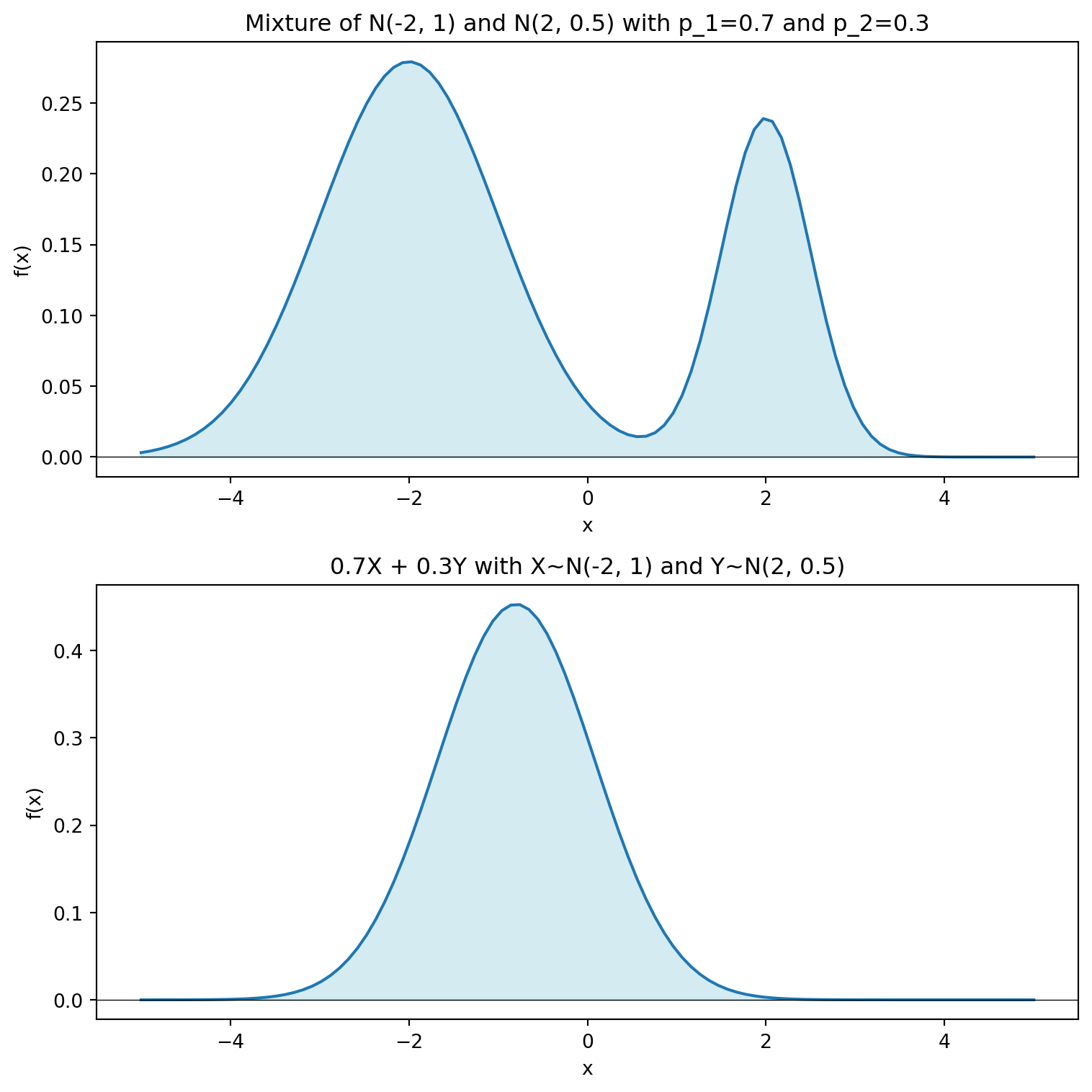
WarningMixture vs Linear Combination
Note that this is not the same as constructing a linear combination of the component distributions. For example, if \(X_1 \sim N(\mu_1, \sigma_1^2)\) and \(X_2 \sim N(\mu_2, \sigma_2^2)\) are independent, then \(w_1 X_1 + w_2 X_2\) is a normal distribution with mean \(w_1 \mu_1 + w_2 \mu_2\) and variance \(w_1^2 \sigma_1^2 + w_2^2 \sigma_2^2\). This is not the same as a mixture of two normal distributions, which would be bimodal if \(\mu_1\) and \(\mu_2\) are sufficiently different.